in the Broadest Sense
June 2002
Abstract
The main purpose of this project is to explore mathematical models of dynamic behavior. The content of this exploration will hopefully provide a clear and basic overview of the fundamental concepts of complex dynamic systems and the transformations that may occur within such systems. The primary motivation for this type of endeavor is the fact that most of the problems we, the human species, are facing today cannot be overcome unless we are collectively able gain a general familiarity with the complicated dynamic patterns of change which are present everywhere in nature. Indeed, the present frontiers of science and human understanding, especially within the branches of physics, sociology, neuroscience, economics, biology, and engineering, all have one thing in common. Within all these areas of human research, we are struggling to come up with metaphors and analogies that sufficiently represent the basic properties of nonlinear chaotic behavior within higher dimensional systems.
Dynamic Systems Theory
The field of dynamics is a vast subject whose origins can be traced back roughly four hundred years to the time of Newton, Galileo, and Kepler. There were actually very few significant advances throughout the next few hundred years until the beginning of the 20th century when new breakthroughs were made by Poincare and Liapounov. At this time, the study of dynamic behavior was primary concerned with the analytic properties of various mathematical functions.
These functions served as simple models whose behavior reflected certain types of physical phenomena such as pendulums, falling bodies, and spring-mass systems. In most cases, the analytic approach to modeling a natural system involves two basic steps. Firstly, model builders have habitually used techniques which allow for an extremely complex higher dimensional system to be collapsed into a lower dimensional toy model. Secondly, the equations for these models often contain nonlinear terms, which can lead to serious difficulties in mapping the dynamics of the system. These nonlinear terms are usually linearized using a functional approximation.
These two steps allow mathematicians to work out problems by hand in a reasonable amount of time. If a system is not low dimensional or linear, it is usually very frustrating to use the analytic approach. The basic idea used for analyzing nonlinear dynamic systems involves finding the equilibrium values, and then trying to determine the behavior of the system for values in the local neighborhoods of each equilibrium. However, it is often quite impossible to determine the behavior of the system for values between these local neighborhoods.
The limiting features of the analytic approach were dramatically overcome during the 1960’s with the advent of computer technologies. The power of computers in modeling dynamic systems lies in their ability to process astronomically large numbers of calculations in a relatively short amount of time. This new technology led to an alternative approach for modeling the behavior of complicated systems. Instead of solving the equations analytically, dynamicists are now able to obtain geometric images that represent the qualitative patterns of change within the system. The evolution of the system in time is represented by a family of trajectories, or curves, in an abstracted mathematical space. The basic dynamic properties of the system are revealed by observing the limit behavior of these trajectories as time goes to infinity.
Before we delve any further into this exploration, let’s define a dynamic system. In general, a dynamic system can be defined as any pattern of change. The system can be open or bounded, continuous or discrete, conservative or dissipative, finite or infinite dimensional. Mathematically, we can make our definition more specific. Let S be the space of all possible states of the system. This mathematical space, commonly called state space, is usually an open subset of Euclidean space characterized by Cartesian coordinates. A dynamic system is a rule, or function, which represents how the states of the system, or points in state space, change in time. Let us define the following.
| Definition: φ t : S → S is a dynamic system if φ t is a C 1 function and S = state space = { x | x ∈ possible state of the system }. The change within the system, with respect to time, is represented by d/dt φ t , such that d/dt φ t = x = f (x), where f (x) is a system of equations. | |
For
example, f (x) = { |
dx1/dt = f1 ( x1, x2, . . . . . ., xn ) | |
| dx2/dt = f2 ( x1, x2, . . . . . ., xn ) | ||
| . . | ||
| . . | ||
| dxn/dt = fn ( x1, x2, . . . . . ., xn) |
In this context, the function, f (x), generates a vector field, in which a vector is assigned to every point in the state space. The function φ t is C 1 if it is continuously differentiable at all points x. The dimension of the state space, n, is the least number of variables necessary to completely describe the system under investigation. This number is also referred to as the degrees of freedom within a system. The general solution to a system of differential equations is a family of integral solution curves which fill the entire space and are all tangent to the directional vectors at each point. These curves are usually called flow lines. It is impossible to draw all of these flow lines, but by drawing only a handful it is possible to grasp the entire behavior of the system for different initial conditions. This image of the state space along with a collection of flow lines is called the phase portrait representation of the dynamic system. A single solution curve, or flow line, which passes through a point x is usually represented as φ t (x), -∞ ≥ t ≥ ∞ . This single trajectory is called a particular solution of the system, and is determined by the choice of initial conditions.
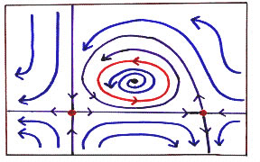
FIGURE 1: 2D phase portrait
If the system is dissipative (i.e. if there is some type of friction or damping), then, as time approaches infinity, the trajectories in state space will be attracted toward some type of limit behavior. These attracting limit sets, or attractors, are the fundamental objects in dynamic systems theory. Surprisingly, there are only three possible types of attracting limit sets.
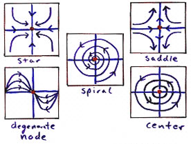
The simplest type of attractor is the fixed point, also called a static equilibrium. If a point x is a fixed point then it must also satisfy the following equation: f (x) = 0. This means that the rate of change of the system at x equals zero. If we chose this point as an initial condition, then the system will remain in that state for all time. Also, other initial conditions will produce trajectories which are usually either attracted toward or repelled away from a fixed point. There are ten basic forms of fixed points. The figure below illustrates five of these in two dimensions. The other five forms can be produced by reversing the arrows in each phase portrait. Also, these forms have analogues in all higher dimensional state spaces.
The second type of attractor is the periodic cycle, also called a limit cycle. This type of behavior is characterized by a closed loop in state space. Periodic cycles are commonly used to model simple oscillators. If a point x lies on a periodic cycle then it must also satisfy the following equation: f (t, x) = f (t + T, x) where T is real number which represents the period of the cycle. In other words, if we chose an initial condition which lies on a periodic cycle, then the flow line which originates from x will return to x after some interval of time T. This means that the state of the system changes in time, but repeats the same pattern over and over for all time. Periodic cycles, like fixed points, can be either attracting or repelling.
Until researchers started using computer modeling techniques during the 50’s and 60’s of the last century, fixed points and periodic cycles were the only recognized forms of possible limit behavior. With the exception of a few pioneers, including Poincare, many people believed that if the system did not contain a fixed point or a periodic cycle, then the behavior of the system must be random. However, with the aide of computers, researchers discovered a new type of limit attractor which was neither a fixed point, a periodic cycle, nor a random trajectory. This new type of behavior, which was predicted by Poincare, is what we now refer to as chaos.
A chaotic attractor is the limit set of a bounded, aperiodic trajectory. In other words, a chaotic trajectory does not escape to infinity nor does it ever return to a point in state space that has already been visited. As time goes to infinity, this chaotic trajectory will trace a very complicated pattern which eventually fills some region of state space. The limit set of a chaotic trajectory is a fractal precisely because it remains bounded, and yet the pattern never repeats. The image below illustrates a chaotic attractor which was discovered by Lorenz.
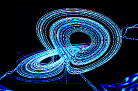
FIGURE 3: Lorenz Attractor
Another feature of chaotic attractors is extreme sensitive dependence on initial conditions. This means that if we choose two initial conditions, which are very close to each other, and then we follow their trajectories in time, the distance between these trajectories will usually diverge exponentially. However, instead of flying off to infinity, they will race around the fractal structure of the chaotic attractor. In a relatively short amount of time the location of each trajectory could end up anywhere within the attractor. Because of this inherent property of chaos, long-term prediction becomes entirely impossible, primarily because it is impossible to take perfect measurements. Experimental mathematicians are often successful in predicting the general locus of possible states for which the system is likely to realize; however, it is usually impossible to guess exactly what state the system will be in for any arbitrary instant in time.
In general, dynamic systems contain multiple attractors. These systems are often referred to as being of the “garden variety.” This is because the state space representation is composed of various areas, which exhibit different forms of dynamic behavior. Each attractor, whether it’s a point, a period, or something else, has a certain range of influence. In other words, different initial points will end up traveling toward different attractors. The set of points in state space, which are attracted to a given attractor, is called the basin of attraction for that attractor. Every attractor comes with it’s own basin. In addition, the union of all of the basins will be exactly the entire state space.
The set of points which forms the boundary between two or more attractors is called a separatrix The separatrix is a repelling set, which is comparable to the peak of a mountain range. If you are able to balance on the peak, fine. However, if you lean a little bit to either side, you will roll down into one the many valleys, or attractors. A separatrix can be a one dimensional curve, a higher dimensional surface, or a thick fractal. In the case of a fractal separatrix, the basins of competing attractors are mixed together and totally interpenetrate each other. The figure below illustrates a fractal separatrix for a periodically forced double-well oscillator
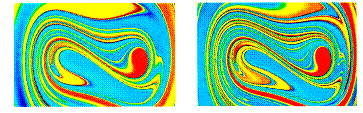
FIGURE 4: fractal separatrix
The specific details of phase portrait representations vary widely between differing systems of dynamic functions. For example, there are infinitely many types of closed curves, but each of them represents a periodic cycle. If we deform the phase portrait, we can obtain a simplified image of the dynamic behavior which is topologically equivalent to the specific phase portrait representation. Two phase portraits are topologically equivalent if there exists a homomorphism between the functions of the two systems. A homomorphism is a mapping, σ, from one space into another such that σ(ab) = σ(a) · σ(b), " a, b Î S. In this case, S is the state space. Basically, a homomorphic mapping is a continuous deformation of the phase portrait, which can entail bending and warping; however, ripping and tearing of the patterns in phase space would violate the condition for topological equivalence. This new abstracted version of a system is sometimes called the superdynamic representation of the system. The superdynamic is simpler than the phase portrait because folded up closed curves become regular circles, and multiple fixed points can be lined up along an axis by rotating the entire coordinate reference frame.
Bifurcation Theory
The superdynamic can visually convey the entire pattern generated by the dynamic rule of the original system, or of any system which is homomorphic to the original system. Usually, if the patterns are intended to represent state changes in time, the dynamic rule is a system of ordinary differential equations. These equations often contain terms with variable coefficients, which are often referred to as control parameters of the system. That is, if the function is a model of a some physical phenomena, then a variable coefficient represents some qualitative attribute which can vary over some range of values. A parameter is analogous to a knob, or dial, which can be turned to different positions.
Each specific value of a control parameter corresponds to a specific superdynamic representation of the system. If we modulate the value of a parameter, the patterns of the superdynamic change as well. A model with control parameters is called a dynamic scheme. The most common representation of a dynamic scheme is a parameterized family of dynamic systems, where each parameter value corresponds to a single dynamic system, or superdynamic. A specific superdynamic is a single slice of the whole dynamic scheme. This new form of abstracted mathematical space is called parameter space, and the pattern formed in this space is called a response diagram. By viewing the system in this way, it is possible to observe the qualitative changes of the system’s behavior as a parameter value is varied.
Usually, the patterns of flow lines in state space change smoothly if the parameter is also changed smoothly. In this context, a smooth transition is again referring to the concept of topological equivalence. Two slices of the response diagram are topologically equivalent to each other if one can be obtained from the other by applying a continuous deformation of the superdynamic.
Interestingly, the adjacent superdynamics in the response diagram are not always topologically equivalent to each other. In other words, as a parameter crosses some critical value, a qualitative change may occur in the dynamic behavior of the system. These critical values are also called bifurcation points. A bifurcation is an event, which is characterized by the occurrence of a dynamic transformation within the system. Even if a parameter is varied slowly, the superdynamic representations of the system before and after the bifurcation event can be dramatically different from each other. Bifurcation theory is the study of how a superdynamic transforms as a number of control parameters are varied.
For this project, we will be primarily interested in exploring examples of elementary single-parameter bifurcations. More complicated bifurcation events are possible if we vary more than one parameter value at the same time. In order to study single-parameter bifurcations, we simply hold all of the parameters constant except for the one that we want to investigate. There are infinite variations of possible bifurcation events; however, these numerous bifurcations can be broken down into three characteristic categories. The three basic types of transformations are subtle bifurcations, catastrophic bifurcations, and explosive bifurcations.
The first type of bifurcation category is called subtle because the transformation of the superdynamic is smooth in the sense that the changes are not immediately striking. The simplest example of a subtle bifurcation, called the first excitation, was rigorously explored by Eberhard Hopf in 1942. This event, which is now commonly called a Hopf bifurcation, involves the transformation of a fixed point into periodic cycle. That is, for some parameter value, the superdynamic contains a fixed point. As the parameter is varied, this fixed point may move around in state space. When the parameter value reaches the critical point, the fixed point switches stability and emits limit cycle. In a supercritical Hopf bifurcation, an attracting fixed point becomes repelling, and an attracting cycle is created. In a subcritical Hopf bifurcation, a repelling periodic cycle becomes a repelling fixed point. The figure below demonstrates the supercritical Hopf bifurcation in two dimensions.
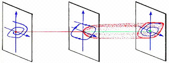
FIGURE 5: first excitation
Another example of a subtle bifurcation is the second excitation. This bifurcation, which is analogous to the event described above, is sometimes called the secondary Hopf bifurcation. In the supercritical case, demonstrated below, an attracting periodic cycle expands to become an attracting invariant tori (AIT). In the subcritical case, a repelling tori collapses into a repelling periodic cycle.
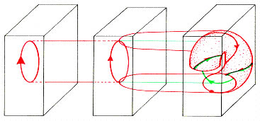
FIGURE 6: second excitation
The second category of bifurcations include events which are called catastrophes. A catastrophic bifurcation usually involves the appearance or disappearance of an attractor along with its entire basin. The case of a disappearing attractor usually occurs when an attractor drifts toward the boundary of its own basin. When the attractor reaches the separatrix, the attractor, the basin, and the separatrix all disappear into thin air.
The simplest type of catastrophe is the one-dimensional static fold, illustrated below. In this example, a one-dimensional state space contains an attracting fixed point and a repelling fixed point. As the parameter value is varied, these equilibrium points move closer and closer together. At the critical value, these points meet and annihilate each other. After the bifurcation event there are no more fixed points. This static fold catastrophe can also be found in two-dimensional systems. In this case, an attracting fixed point and a saddle point approach each other and annihilate when they touch.
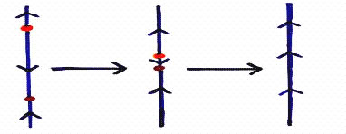
FIGURE 7: 1D static fold
These types of static fold bifurcations for continuous systems are analogous to several types of bifurcations which are often encountered in the study of discrete iterative maps. These events include, the pitchfork bifurcation (an attracting point becomes repelling and emits two attracting points), the transcritical bifurcation (two points collide and switch stabilities), and the saddle-node bifurcation (an attracting point and repelling point annihilate each other).
Another bifurcation that can occur in dynamic systems, which have at least two dimensions, is the periodic fold catastrophe. This bifurcation event involves two periodic cycles which have opposite stabilities. Typically, an attracting cycle and a repelling cycle move toward each other until they collide, at which point the cycles are annihilated.
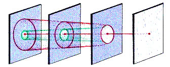
FIGURE 8: 2D periodic fold
The third class of bifurcations include events which are called explosions. An explosion is typically characterized by a sudden and dramatic expansion, or contraction, in the size of an attractor. The simplest example of an explosion is something called the blue loop bifurcation. Before the bifurcation event, there exists an attracting fixed point. At the bifurcation point, a limit cycle appears, but instead of expanding from the original fixed point as in the Hopf bifurcation, the fixed point instantly becomes the full-blown limit cycle. Whereas the blue loop is an example of a fixed point which explodes into a periodic cycle, there are other cases of explosive bifurcations where a periodic cycle explodes into a chaotic attractor. There are also cases in which a small chaotic attractor instantly explodes into a very large chaotic attractor, or vice versa.
Up until this point, we have only considered bifurcation events that occur at a single, very unique, critical value. However, in many complex systems, it is common for a dynamic scheme to contain a large number of such critical values. Often times, there are actually an infinite number of these critical values, which are distributed along the response diagram in a very thick fractal pattern. Sometimes, the entire set of infinitely many bifurcation points is regarded as a single bifurcation event These types of bifurcations are called fractal bifurcations.
Now that we’ve explored some of the basic bifurcation events, it might be helpful to go back and summarize the various levels of abstraction that we have been using to represent the dynamic behavior of a given system. The first level is just the physical system itself. This system could be any physical phenomena which occurs in nature. The next level is the basic mathematical representation of the dynamic system in terms of a system of differential equations. This level of abstraction, called the phase portrait representation, includes the directional vector field generated by the function as well as the flow lines in state space.
The third level of abstraction is what we’ve been calling the superdynamic representation. The superdynamic is an abstraction of the phase portrait which takes advantage of the idea of topological equivalence. For example, any type of bended closed curve can be deformed into a regular circle. The fourth level of abstraction is the dynamic scheme representation, in which each value of a control parameter corresponds to a specific superdynamic. These superdynamics are then placed side by side to create the response diagram. Placing the system in this abstract frame of reference is a very powerful tool which allows a dynamicist to visually analyze the dynamic properties of a given system.
The primary feature of the response diagram is the location of the critical bifurcation points. In order to get a better idea of what these points represent physically, we should consider the concept of structural stability. First of all, this idea is directly related to perturbation theory, in which dynamicists study the effects, on a system, of small changes in the value of a control parameter. If the behavior of the system remains qualitatively the same, as a parameter is varied, then the system is considered stable. However, we’ve already seen that the dynamics before and after a bifurcation are not qualitatively similar. Qualitatively similar is another way of saying topologically equivalent. In other words, the bifurcation points are points where the dynamic system becomes structurally unstable.
For an example, let’s consider the basic Hopf bifurcation. At the critical value, there exists only one fixed point; however, if the parameter is increased beyond this critical value, even if the perturbation is infinitesimally small, then there exists a periodic cycle, which is definitely not topologically equivalent to a fixed point. Generally speaking, at the instant of the bifurcation event, the previously stable pattern of dynamic behavior ceases to exist. Beyond the threshold of this event, new types of behavior emerge.
Dynamics of Superspace
This concept of structural stability can be illustrated quite easily by taking the dynamic scheme representation to the next level of abstraction. Previously, we have associated each superdynamic with a single slice of the response diagram. Now, we will represent every superdynamic, of a given system, as a single point in a new type of mathematical space. This space can be called superspace. As a paramter value is changed, a curve is generated in superspace which represents the changing superdynamic.
At the bifurcation point, the curve intersects with a surface which is called the bad set. The bad set consists of all dynamic systems which are not structurally stable. The following image shows two slices of the response diagram for a Hopf bifurcation, and it also shows the points in superspace which represent these superdynamics. The blue curve represents the entire response diagram, and the red surface represents the bad set.
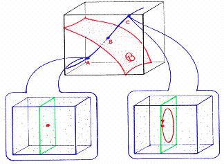
FIGURE 9 : Superspace
We’ve already mentioned that it is typical for a complex dynamic system to have many bifurcation points. When these critical points are in close proximity to each other, the bad sets accumulate in fractal layers of surfaces. The next illustration demonstrates two generic superspace representations in which a fractal bifurcation occurs.
|
|
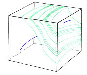
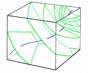
FIGURE 10: Fractal Bifurcations in Superspace
Typically, a curve in superspace is an abstract representation of a dynamic system which changes and transforms as a single control parameter is being varied. However, in a broader sense, the curve may represent any system for which the dynamic rule is changing continuously in time. The function, which describes this curve, can be expressed as Ωt (x). This type of definition is similar to our original formulation of a dynamic system. Remember, each point in state space represents a single state of the system. The time evolution of a single state was represented by φt (x), which is a particular solution to the system of differential equations d/dt φt. The general solution, which is the overarching dynamic rule of the system, was represented simply as φt . In superspace, each point represents an entire dynamic system, or superdynamic. The time evolution of an entire system is now represented as Ωt (x), -∞ ≥ t ≥ ∞.
Our motivation for building this model is that we want to illustrate the mathematical representation of a system which is continuously transforming. Usually, dynamic systems theory focuses primarily on systems which are characterized by a fixed function. Since the general solution of the system often contains variable parameters, it becomes necessary to explore what happens at different parameter values in order to fully map the dynamic landscape which is generated by the original system. However, we are now describing a system which is evolving in time. A simple example of this in nature is the growth and development of a human being from birth to death. Within this interval of time, the dynamic system of the physical/emotional/spiritual body transforms a number of times from childhood, through adolescence, into adulthood, and then into old age. Another example is the evolution of an entire species over many eons. In this case, the genetic program evolves over a period of time that is much longer than the lifespan of any one organism within the species. We are using the expression Ωt (x) because the evolving system can be thought of mathematically as a trajectory, or flow line, in superspace.
It may be reasonable to suppose that there exists some organizing principle which influences the unfolding pattern of an evolving system. It is hypothesized here that the evolutionary trajectory of a natural system may be one particular solution of a much larger system. For example, let’s consider a model in which a potential field, or vector field, is defined over some open subset of superspace. This field can be expressed as d/dt Ωt , and the general solution to this new type of system can be expressed as Ωt . At this stage of model building, it is relatively unimportant whether or not we could actually find this function analytically. What is important is that the general solution of d/dt Ωt generates a whole family of solution curves which fill an entire subset of superspace. In other words, for different initial conditions, this vector field will generate many different types of evolutionary trajectories.
This new type of dynamic system can be expressed simply as Ωt : S → S, where S is the space of all possible superdynamics. Since each superdynamic, or point in superspace, is a characterized by a function, it seems natural to use function space as our standard frame of reference. Function space is very interesting because it is an infinite dimensional space. Thus, a particular solution of d/dt Ωt will be a trajectory in function space.
Given the concepts which have already been addressed, it also seems natural to expect that these trajectories in superspace may exhibit various forms of limit behavior such as fixed points, periodic cycles, and chaotic attractors. As an example, let’s consider the case of an attracting fixed point. First we choose an initial condition, which is a point in superspace. If we follow the time evolution of this point, as determined by Ωt , the trajectory will approach the attracting fixed point. As time goes to infinity, the dynamic rule, or function, of the initial superdynamic converges to another particular function. Alternatively, if there exists a single chaotic attractor in superspace, then the dynamic rule of the initial superdynamic never settles down into a stable configuration. Instead, the function flies around the chaotic attractor on a trajectory that never repeats itself. If there are more control parameters for this superspace system, then we can also expect to encounter various analogues of all the bifurcation events that have been discussed in this project.
This model is designed to be able to illustrate how a large number of evolutionary systems may be generated from a single overarching dynamic system. In other words, many seemingly separate evolutionary systems, or patterns, may all be specific aspects of one system which exists on a higher dimensional level. As a simple example, let’s consider the dynamic system which is the entire planet Earth. Within this system there are many different types of evolving species. Although the evolution of the human race and the evolution of a particular insect species may seem unrelated, they are actually both expressions of the same planetary system, that is, they are each particular solutions of one whole system.
However, it would be naïve to assume that the dynamic system of the entire Earth is unchanging. That is, it seems probable that the planet Earth is itself an evolving dynamic system. Just as before, we can represent this evolving system as a trajectory in an even higher dimensional superspace. The evolution of a planetary system, in this context, could be a particular solution of the dynamic system which is the entire solar system. An evolving solar system can be represented as a specific aspect of the entire galactic system. In general, each time we allow the overarching dynamic rule of a system to evolve, we can collapse this evolutionary progression into a single trajectory which lives in a new level of abstracted superspace. Interestingly, since we’ve defined superspace to be the space of all possible superdynamics, and since every possible evolutionary system is, hypothetically, a specific solution of an even higher dimensional superdynamic, it is possible that all these systems could be represented as nested levels within one infinite dimensional superspace. In this context, the system Ωt is considered to be the universal dynamic system of all that is.
Quantum Chaos
The systems which we’ve been considering so far have all been characterized by deterministic equations. Let’s now incorporate a probabilistic model into our toolbox of dynamic metaphors. The primary motivation for this is that the dynamic rule which describes an evolving superdyanmic may actually be a probabilistic function. The task of describing this probabilistic function should be relatively easy because we have already reached the infinite dimensional level of function space. In quantum theory, the instantaneous state of a quantum system is represented mathematically by a point in what is called Hilbert space. Hilbert space is a complete function space on which a norm is defined. This mathematical jargon basically means that the space is filled with points, and that we have created some standard unit of measurement, which we call the norm.
First, let’s summarize the basics. A quantum state, represented by Ψ, is a wave of possibilities. The number of possibilities for some systems may be small, but typically there exists an uncountably infinite number of possibilities. Each distinct possibility is represented as a single dimension of Hilbert space. However, in this context, each dimension of Hilbert space is a complex plane, not a real line. The wave function, Ψ, assigns a specific coordinate value to each dimension in Hilbert space. Conversely, any arbitrary point in Hilbert space, Ψo , can be expressed as a linear combination of terms such that each term contains a coordinate value from one of the dimensions.
Since each dimension is a complex plane, the coordinate value for each dimension can be expressed as a complex number in polar form; i.e. z = re iθ . In this way, each coordinate value is characterized by two numbers, r and θ. These numbers represent the amplitude and phase values which correspond to a specific possibility. In other words, the wave function, Ψ, is the sum of a bunch of possibilities, where each possibility is a wave that has an amplitude and a phase. In quantum theory, the square of the amplitude value for each possibility is a measure of how probable it is for that possibility to occur. This probabilistic function, Ψ, can be written in the following way: Ψ = ∑ ciΦi, where c is a complex coordinate value along a specific dimension, Φi. Also, the sum of all our probabilities must equal one, i.e. ∑ ci2 = ∫ || Ψ(x) ||2 dx = 1.A quantum state is represented in Hilbert space by a vector which extends from the origin and whose endpoint is at the location of Ψ. In a way, the function Ψ is analogous to a probabilistic attractor. That is, there exists a set of possibilities, and some of these possibilities are more likely to occur than others. In a typical chaotic attractor, the trajectory of a point may visit some areas of the attractor more often than others; thus, certain regions have a higher probability density.
The next step in constructing this model is to consider how the Ψ-wave changes in time. In general, the individual coordinate values for each dimension vary as time progresses. As these values change, so does the orientation of the vector which represents the quantum state of the given system. This spinning vector traces a parameterized curve, in Hilbert space, which can be represented by Ψt. In other words, Ψt is the pattern generated by a continuously morphing probabilistic attractor.
Typically, the time evolution of Ψt is expressed using the Schrodinger equation; however this equation is linear, and therefore the solutions, qualitatively, will always be nice and simple. In our case, we are trying to build models which can be used to represent any abstract natural system. Generally, these natural systems are very hyperdimensional and incredibly nonlinear. Thus, we will abandon the Schrodinger equation and all of its linear analogs.
If the dynamic rule which governs the evolution of the Ψ-wave is nonlinear, a feature that was implicitly assumed in our earlier formulation of Ωt in superspace, then we are likely to encounter all the familiar objects of dynamic systems theory. That is, we are likely to find fixed points, periodic cycles, chaotic attractors, basins, and separatrices. We may also encounter cases in which the limit behavior of the probabilistic system transforms in some type of bifurcation event. In fact, if we intend to use this model to describe the incredibly complex dynamic patterns which are found in natural systems, we are likely to encounter an uncountaably infinite number of chaotic attractors and bifurcation events.The basic idea is that the evolution of natural systems can be represented qualitatively in terms of morphing fields of probabilistic tendencies. If we apply the concepts which were developed in the previous section, it becomes theoretically possible that the dynamic rule which generates these evolving probabilistic systems may itself be evolving probabilistically. It is now also theoretically possible to consider the likelihood that these infinite levels of nested probabilistic systems are integral aspects of one infinite dimensional superspace system. This abstract system, which we have been conveniently referring to a Ωt, represents the universal superdynamic system which is responsible for the generation and evolution of all possible dynamic systems which occur in nature, not excluding the minds of seriously disturbed mathematicians such as myself.
In the beginning of this exploration we discussed the analytic approach to modeling dynamic systems, and we addressed the fact that it is generally impossible to solve even simple lower dimensional nonlinear systems using this method. It is ludicrous to think that any human mathematician would ever be able to solve for a system as incredibly complex as the Earth, let alone be able to solve for our abstract universal system Ωt. However, solutions to these systems exist everywhere around us within the patterns generated by nature. Instead of beating our heads against a wall trying to describe these patterns using analytic functions, it might be a good idea to explore these complex dynamic systems using artistic audio/visual representations, which may be able to convey the essential features of a system through an actual subjective experience of reality as opposed to the objective experience of some dusty chalkboard filled with unintelligible symbols. The information within this project is not intended to be conclusive or mathematically rigorous. The purpose is simply to explore new dimensions which are beginning to appear on the cusp of the exponentially expanding field of dynamic systems theory. Let’s conclude our exploration with some visual images which have been obtained using computer simulation technologies specifically programmed to illustrate some of the concepts that have been addressed within this project.
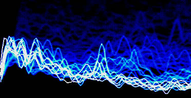
FIGURE 11: An abstract representation of a morphing probabilistic quantum wave
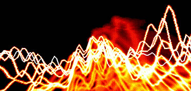
FIGURE 12: Another morphing quantum wave
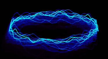
FIGURE 13: A morphing quantum wave which forms a periodic cycle
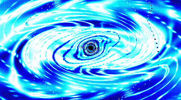
FIGURE 14: Quantum Attractor
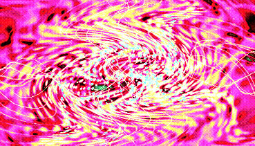
FIGURE 15: Quantum Attractor
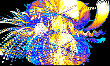
FIGURE 16: Quantum Attractor
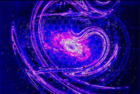
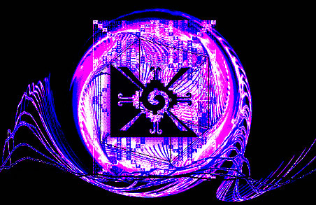
FIGURE 17: Galactic Love Attractor
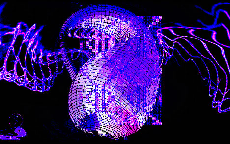
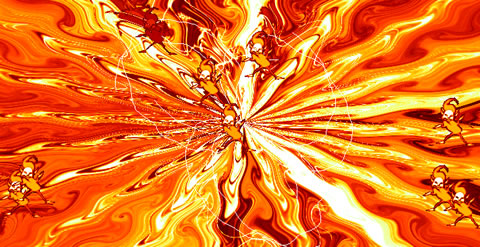
FIGURE 18: Infinite Source Attractor
Sources & Sinks
Abraham, Ralph. Dynamics – The Geometry of Behavior: Part 4. Aerial Press, Inc. Santa Cruz. 1988.
Arnold, Vladimir. Catastrophe Theory. Springer-Verlag. 1984,
Awrejcewicz, J. ed. Bifurcation and Chaos. Springer-Verlag. 1995.
Capra, Fritjof. The Web of Life. Anchor Books. 1996.
Demazure, Michel. Bifrucations and Catastrophes. Springer-Verlag. 2000.
Herstein, I. N. Topics in Algebra. John Wiley & Sons. 1975.Kuznetsov, Yuri. Elements of Applied Bifurcation Theory. Springer-Verlag. 1995.
Smale, Stephen, & Hirsch, Morris. Differential Equations, Dynamic Systems, and Linear Algebra. Academic Press. 1974.
Stogatz, Steven. Nonlinear Dynamics and Chaos. Perseus Publishing. 1994.
Verhulst, Ferdinand. Nonlinear Differntial Equations and Dynamic Systems. Springer-Verlag. 2000.
*** Special thanks to Ralph Abraham and Chris Shaw for the use of figures 5, 6, 8, 9, & 10.